Database Systems
Summary
Summary
Table of Contents
- Data vs Information
- File processing systems vs databases
- Entities and relationships
- Constraints
- Weak Entity
- Ternary relationships
- Attributes
- Relational Data Model
- Keys
- Integrity constraints
- ER to Relational model
- Conceptual to logical checklist
- Convert from Logical
- Basic Operations
- Compound Operators
- SQL
SELECTstatement overview- Other Statements
- Views
- More DDL
- Approach for writing SQL
- Files in DBMS
- Indexes
- Query Processing
- Relational Operations
- Projection
- Joins
- Query plan
- Query optimisation steps
- Single-relation plans
- Multi-relation plans
- Motivation for Normalisation
- Functional dependency
- Steps in Normalisation
- Normalisation vs Denormalisation
- Capacity Planning
- Backup and Recovery
- Backup Taxonomy
- Backup Policy
- Transactions
- Concurrent Access
- Transaction Log
- Data Warehousing
- Dimensional Modelling
- Distributed Databases
- Distribution Options
- Comparing configurations
- Functions of a distributed DBMS
- Date’s 12 Commandments for Distributed Databases
- Motivation for NoSQL
- NoSQL Goals
- Object-relational impedance mismatch
- 3Vs of Big Data
- Big Data Characterisitics
- NoSQL Features
- NoSQL Variants - Aggregate oriented
- NoSQL Variants - Graph databases
- CAP Theorem
- ACID vs BASE
1. Databases
Data vs Information
- Data: known facts, stored and recorded e.g. text, numbers, dates, …
- Information:
- data presented in context.
- may be summarised/processed.
- increases user knowledge.
- Data is known and available; information is processed and more useful
- DBMS: software designed to store, manage, facilitate access to databases
File processing systems vs databases
File processing systems
- data duplication: wasteful
- program-data dependence: program needs to change if file structure changes
- poor data sharing
- high program maintenance
- long development time
Database systems
- data independence: separate data from program
- minimise data redundancy
- improve data consistency
- improve data sharing
- reduce program maintenance
- ad hoc data access via SQL
2. Database development lifecycle
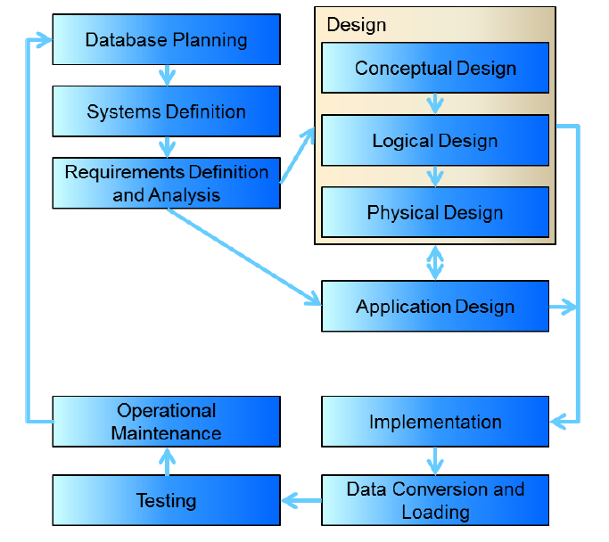
- Planning: how to do project
- how enterprise works; top level perspective on data requirements
- enterprise data model
- Systems definition: specify scope and system boundaries
- who are the users, what is the application area
- how does system interfere/interact with other systems
- Requirements definition and analysis: collection and analysis of requirements for the new system
- Conceptual design: construct model of data independent of physical
considerations
- Identify business rules
- ER entity-relationship diagrams
- Logical design
- relational model of data based on conceptual design
- independent of specific database
- foreign keys
- cardinality
- Physical design: description of implementation of logical design for a
specific DBMS
- data types: help ensure consistency, integrity, minimise storage space
- need to consider range of possible values and data manipulation required
- file organisation
- indexes
- look up/go between tables
- whether or not to perform normalisation/de-normalisation
- denormalise: improved performance; increased storage requirements; may reduce data integrity/consistency
- data types: help ensure consistency, integrity, minimise storage space
- Application design
- design of interface and application
- programs that use/process database
- Implementation
- physical realisation of database
- Data conversion and loading
- transfer existing data into database
- conversion from old systems
- non-trivial
- Testing
- run database to find errors in design/setup
- assess performance, robustness, recoverability, adaptability
- Operational maintenance
- monitoring and maintaining the database
- handling new and changed requirements
3. Conceptual Design
Entities and relationships
- entity: real-world object distinguishable from other objects, described by a set of attributes
- entity set: collection of entities of the same type. All entities in an entity set have the same set of attributes, and is identified by a key.
- relationship: association between two or more entities
- can have attributes
- relationship set: collection of relationships of the same type
Constraints
- key constraints: number of objects participating in the relationship set
- upper bound
- e.g. an employee can work in many departments, a department can have many employees
- one-to-many: represented by an arrow towards relationship set
- participation constraint: whether all entities in a relationship
participate in a relationship
- lower bound
- total participation: all entities must participate; bold line
- partial participation: not every entity need participate
Weak Entity
- weak entity: uniquely identified by considering primary key of owner
entity
- represented by bold rectangle
- identifying relationship also bold
- total participation in identifying relationship
- only have a partial key (dashed underline)
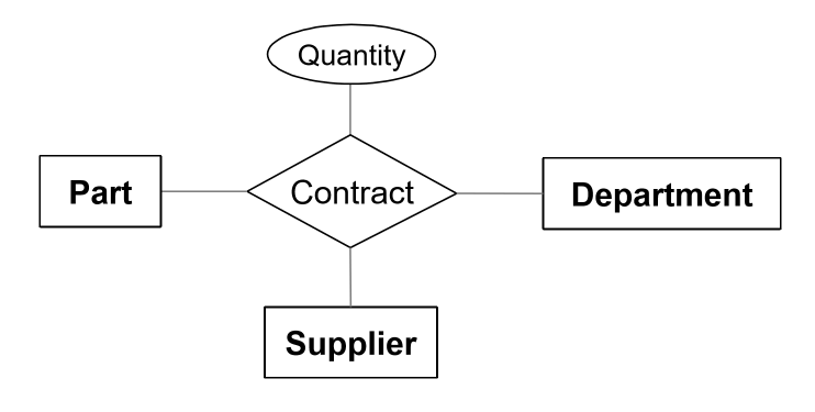
Ternary relationships
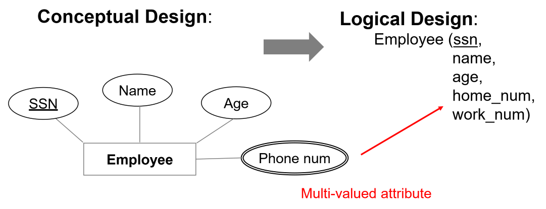
Attributes
- multi-valued attributes: multiple values of same type (e.g. phone numbers)
-
composite attributes: structured values of possibly different type e.g. address
- entity vs attribute: depends on how you use information e.g. several addresses per employee, you should model address as an entity
4. Translating ER diagrams
Relational Data Model
- data model: allows you to translate real world things into form that can
be stored by a computer
- relational, ER, object-oriented, …
- relational model:
- rows: aka tuples, records
- columns: aka attributes, fields
- relational database: set of relations
- relation: schema + instance
- schema: specifies name of realtion, name and type of each column
- instance: table with rows and columns
- cardinality: number of rows
- degree: number of fields
- relation is a set of distinct, unordered rows
Keys
- keys: associate tuples in different relations
- form of integrity constraint: e.g. only students can be enrolled in subjects
Primary key
- superkey: set of fields where no two distinct tuples have the same values for all fields
- set of fields is a key for a relation if:
- it is a superkey, and
- no subset of fields is a super key, i.e. it is a minimal subset
- primary key: chosen key for the relation
- candidate key: all other keys
- each relation has a primary key
Foreign key
- foreign key: set of fields in one relation used to refer to a tuple in another relation. Must correspond to primary key in the other relation
- referential integrity: achieved when all foreign key constraints are enforced
Integrity constraints
- integrity constraint/IC: condition that must be true for any instance of
the database
- specified when schema is defined
- checked when relations are modified
- instance of a relation is legal if it satisfies all specified ICs
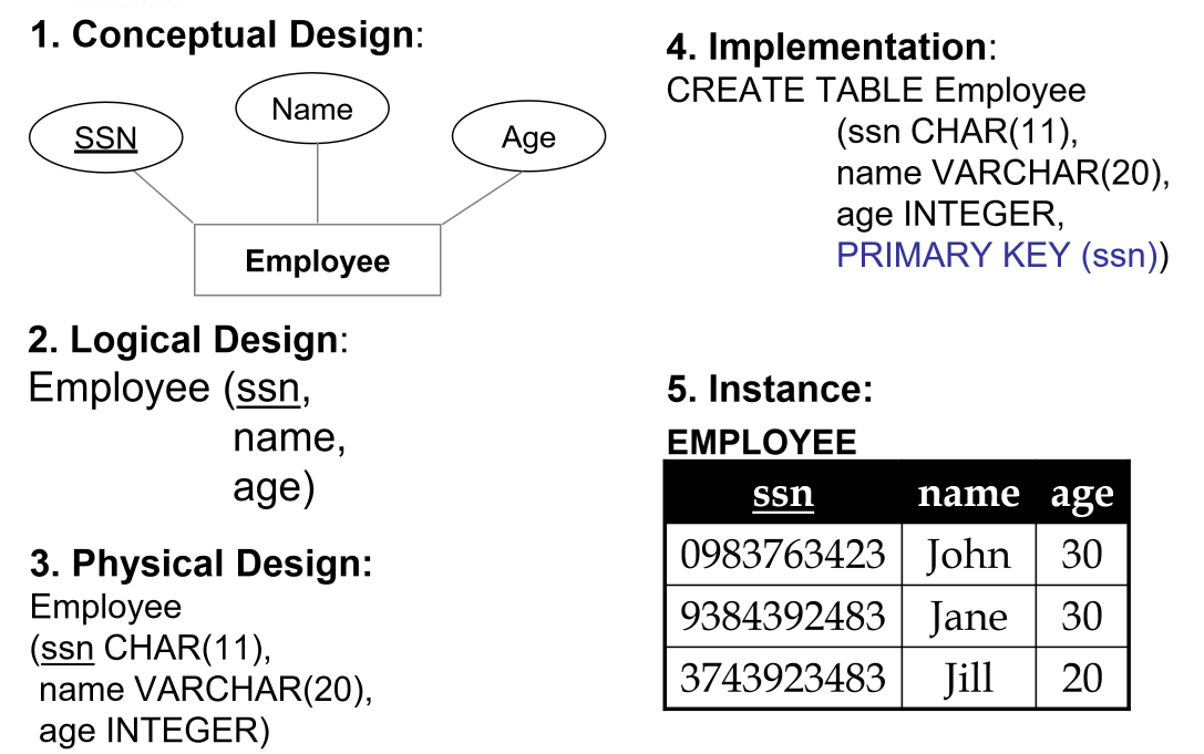
ER to Relational model
- logical design:
- entity sets become relations
- attributes become attributes of relation
- physical design: assign data types
- multi-valued attributes: either flatten or introduce lookup table
- composite attributes: flatten
- many-to-many relationship set to relation
- include keys for each entity set as foreign keys. This will form a superkey
- descriptive attributes
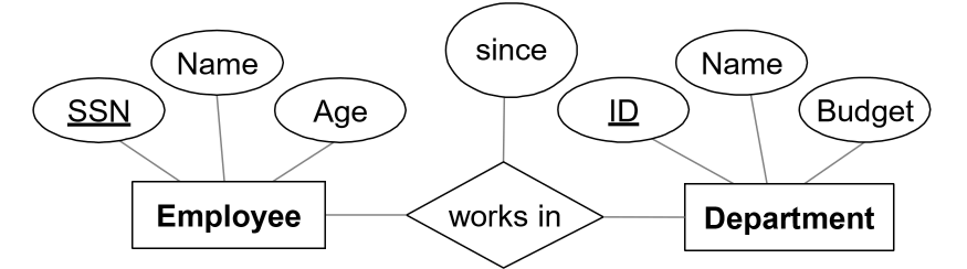
Example
Conceptual design
Logical design
Employee(ssn PK, name, age)
Department(did PK, dname, budget)
Works_In(ssn PFK, did PFK, since)
Physical Design
Employee(ssn CHAR(11) PK,
         name VARCHAR(20),
         age INTEGER)
Department(did INTEGER PK,
           dname VARCHAR(20),
           budget DECIMAL(10, 2))
Works_In(ssn CHAR(11) PFK,
         did INTEGER PFK,
         since DATE)
Implementation
CREATE TABLE Employee (
    ssn CHAR(11),
    name VARCHAR(20),
    age INTEGER,
    PRIMARY KEY (ssn)
);

CREATE TABLE Department (
    did INTEGER,
    dname VARCHAR(20),
    budget DECIMAL(10, 2),
    PRIMARY KEY (did)
);

CREATE TABLE Works_In (
    ssn CHAR(11),
    did INTEGER,
    since DATE
    PRIMARY KEY (ssn, did),
    FOREIGN KEY (ssn) REFERENCES Employee,
    FOREIGN KEY (did) REFERENCES Department
);
Example: key and participation constraints
Conceptual model
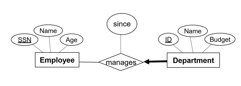
- each department has at most one manager
- rule: primary key from many side becomes foreign key on the one side
- this ensures the key constraint holds
- every department has a manager: total participation. Enforce with
NOT NULL
Implementation
CREATE TABLE Department (
    did INTEGER,
    dname VARCHAR,
    budget DECIMAL(10, 2),
    since DATE,
    ssn CHAR(11) NOT NULL,
    PRIMARY KEY (did),
    FOREIGN KEY (ssn) REFERENCES Employee
        ON DELETE NO ACTION
);
Example: Weak Entity
- weak entity set and identifying relationship set become a single table
- when owner is deleted, all owned weak entities must also be deleted
Logical design
Dependent(dname PK, age, cost, ssn PFK)
Implementation
CREATE TABLE Dependent (
    dname CHAR(20) NOT NULL,
    age INTEGER NULL,
    cost DECIMAL(7, 2) NOT NULL,
    ssn CHAR(11) NOT NULL,
    PRIMARY KEY (dname, ssn),
    FOREIGN KEY (ssn) REFERENCES Employee
        ON DELETE CASCADE
);
5. MySQL Workbench
- derived attributes: values can be derived from other attributes in the
database
- need not be stored physically: redundant, threat to integrity
- may want to store so that you don’t have to recompute
- e.g. number of years employee has been employed
Conceptual to logical checklist
- Flatten composite and multi-valued attributes, or introduce lookup table for multi-valued attributes when number of values is unknown or variable.
- Resolve many-many relationships
- Add foreign keys at crows foot end of relationship (many side)
Convert from Logical
- choose data types
- choose whether
NULLorNOT NULL
Binary relationships
- one-to-many: primary key on one side becomes foreign key on many side
- many-to-many: create associative entity (new relation) with primary key of each entity as combined primary key
- binary one-one relationship: primary key on mandatory side becomes foreign
key on optional side
- otherwise just choose one
Unary relationships
- one-to-one: put FK in relation
- one-to-many: put FK in relation
- many-to-many: generate associative entity
- put two foreign keys in it
Ternary relationship
- generate associative entity
- 3 one-to-many relationships: add FKs
6. Relational Algebra
Basic Operations
- Selection $\sigma$: select subset of rows satisfying selection condition
- result: relation with identical schema to input relation
- Projection $\pi$: retain wanted columns in projection list
- schema: contains only fields in projection list
- eliminates duplicates
- Set-difference $-$: get tuples in one relation but not the other
- input relations must be union-compatible
- not symmetrical: $S1-S2 \not = S2-S1$
- Union $\cup$: tuples in one relation and/or in the other
- input relations must be union-compatible
- duplicates removed
- Cross product $\times$: combine two relations
- each row of one input merged with each row from another input
- output: new relation with all attributes of both inputs
- e.g. num tuples of $S \times R = card(S).card(R)$
- renaming operator $\rho$: useful for naming conflicts e.g. in cross
product
- $\rho(ResultName(\text{ field1 } \rightarrow \text{newField1}, \text{field2} \rightarrow \text{newField2}), S\times R)$
- union-compatible:
- same number of fields
- corresponding fields are of the same type
- or: $\vee$
- and: $\wedge$
Compound Operators
- no additional computational power: they can be expressed in terms of basic operations
- may be useful shorthand
- intersection $\cap$: retain rows appearing in both relations
- inputs must be union-compatible
- $R\cap S = R - (R-S)$
- join: cross product + selection + optional projection
- natural join $R\bowtie S$: match rows where attributes appearing in both
relations have equal values. Omit duplicate attributes. Steps:
- compute $R \times S$
- select rows where attributes in both relations have equal values
- project all unique attributes, copy each common one
- condition join/theta join $R\bowtie_c S = \sigma_c(R\times S)$: cross product with a condition
- equi-join: special case of condition join, where condition only contains equalities
8, 9. SQL
SQL
- Structured Query Language
- Supports CRUD commands:
- Create
- Read
- Update
- Delete
- capabilities:
- data definition language DDL: define, set up database
CREATE, ALTER, DROP
- data manipulation language DML: maintain, use database
SELECT, INSERT, DELETE, UPDATE
- data control language DCL: control access to the database
GRANT, REVOKE
- administration
- transactions
- data definition language DDL: define, set up database
SELECT statement overview
# List columns/expressions returned from query
SELECT [ALL|DISTINCT] select_expr [, select_expr ...]
# tables from which data is obtained
FROM table_references
# filtering conditions
WHERE where_condition
# categorisation of results
GROUP BY { col_name | expr } [ASC | DESC], ...
# filtering conditions for categories.  Can only be used with a GROUP BY
HAVING where_condition
# sort
ORDER BY {col_name | expr | position} [ASC | DESC]
# limit which rows are returned
LIMIT {[offset, ] row_count | row_count OFFSET offset}];
LIKE Clause
%: 0+ characters- ‘_’: exactly 1 character
LIKE "<regex>"
e.g.
SELECT * FROM Customer
# any values starting with "a"
WHERE CustomerName LIKE 'a%'
# any values starting with "a", at least 3 values long
WHERE CustomerName LIKE 'a_%_%'
# any values starting with "a", ends with "o"
WHERE CustomerName LIKE 'a%o'
Aggregate Functions
AVG()MIN()MAX()COUNT(): counts number of recordsSUM()- all except
COUNTignore null values and return null if all values are null
Order By
ORDER BY XXX ASC/DESC
Joins
- Cross product: not usually useful. Typically want records matching on a key
# Cross product
SELECT * FROM R1, R2;

# Natural join: join tables on keys.  Attributes must have same name
SELECT *
FROM R1 NATURAL JOIN R2;

# Inner join: only retain matching rows
SELECT *
FROM R1 INNER JOIN R2
    ON R1.id = R2.id;
k
# Outer join:: left/right; includes records that don't match from the outer table
SELECT *
FROM R1 LEFT OUTER JOIN R2
    ON R1.id = R2.id;
Comparison and logical operators
<>, !=: not equal toIN, NOT IN: test whether attribute is in/not in subquery listANY: true if any value meets conditionALL: true if all values meet conditionEXISTS: true if subquery returns 1+ record
Set operators
- MySQL specific
UNION: classical set operation, no duplicatesUNION ALL: duplicates allowed
Other Statements
INSERT Statement
- insert records into a table
# insert single record
INSERT INTO NewEmployee SELECT * FROM Employee;

# insert multiple records
INSERT INTO Employee VALUES
    (DEFAULT, "A", "address A", "2012-02-12", NULL, "S"),
    (DEFAULT, "B", "address B", "2012-02-12", NULL, "R");

# insert specific columns
INSERT INTO Employee
    (Name, Address, DateHired, EmployeeType)
    VALUES
        ("D", "address D", "2012-02-12", "C"),
        ("E", "address E", "2012-02-12", "C");
UPDATE
- change existing data in table
UPDATE Salaried
    SET AnnualSalary =
        CASE
            WHEN AnnualSalary <= 100000
            THEN AnnualSalary * 1.1
            ELSE AnnualSalary * 1.05
        END;
REPLACE
- works identically to insert, but row is updated if it exists, otherwise a new row is inserted
DELETE
- dangerous!
- in production, you don’t physically delete, you use a flag to indicate not active, known as a logical delete
DELETE FROM Employee
    WHERE Name = "Grace";
- foreign key constraints
ON DELETE CASCADEON DELETE RESTRICT: prevent deletion if child row exists
Views
- view: relation not in physical model, but made available to end user as a virtual relation
- hides query complexity from user
- hides data from users: helps improve DB security
- once created, schema is stored in DB, and it can be used like any other table
CREATE VIEW nameOfView AS validSqlStatement
More DDL
ALTER
- allows you to add/remove attributes from a table
ALTER TABLE TableName ADD AttributeName AttributeType;
ALTER TABLE TABLENAME DROP AttributeName;
RENAME
- allows you to rename table
RENAME TABLE CurrentName TO NewName;
Approach for writing SQL
- Use design as a map to help format queries
- Create skeleton
SELECTstatement as a template - Fill in parts to build query
10. Storage and Indexing
Files in DBMS
- file: collection of pages, each containing collection of records
- each record has a record ID, correspoding to physical address of page that the record is on
- DBMS must support:
- insert, delete, modify records
- read particular records
- scan all records
- pages are stored on hard disks HDD
- for processing, pages need to be loaded into RAM
-
costs of operations modelled by DBMS in terms of number of page accesses (disk I/Os)
- heap files: no order among records
- suitable for retrieval of all records
- as file grows/shrinks pages are allocated/deallocated
- fastest for inserts
- sorted file: pages and records ordered by some condition
- fast for range queries
- hard to maintain: each insertion may reshuffle records
- rarely done in practice; B+ tree index is a better option
- index file organisation: fastest retrieval in some order
- best tool a DBA has to optimise a query
Indexes
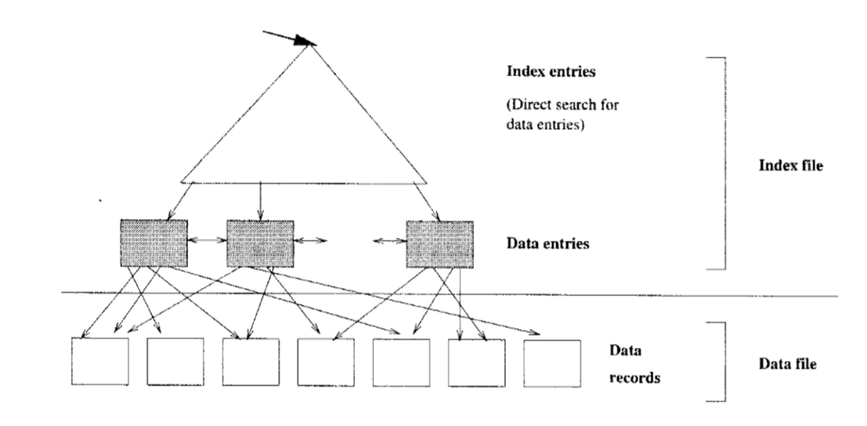
- index: data structure built on top of data pages used for efficient search
- built over search key fields: selections on search key fields will be
fast
- any subset of fields of a relation can be search key for an index
- search key is distinct from key, and need not be unique
- contains collection of data entries, supporting efficient retrieval of data records matching a given search condition
- built over search key fields: selections on search key fields will be
fast
Clustered vs Unclustered
- clustered: order of data records is the same as order of index data
entries
- e.g. if the underlying file is sorted on the same fields
- you cannot have multiple clustered indexes over a single table
- much cheaper for clustered retrieval
- more expensive to maintain
- very efficient for range search
- Cost ~ number of pages in data file with matching records
- unclustered: order of data records is different from order of index data
entries
- e.g. heap file
- cost ~ number of matching index data entries (data records)
Primary vs Secondary
- primary index includes table’s primary key
- never contains duplicates
- secondary index is any other index
- may contain duplicates
Single Key vs Composite Key
- index can be built over a combination of search keys
- data entries in the index are sorted by search keys
Index Type
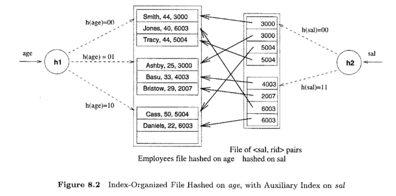
- hash-based index: index is a collection of buckets
- hash function maps search key to corresponding bucket
- h(r.search_key) = bucket in which record r belongs
- good for equality selections
- bad for range selections
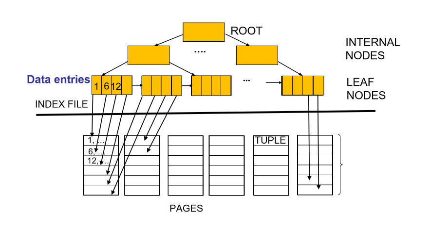
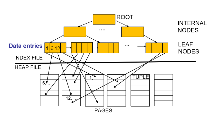
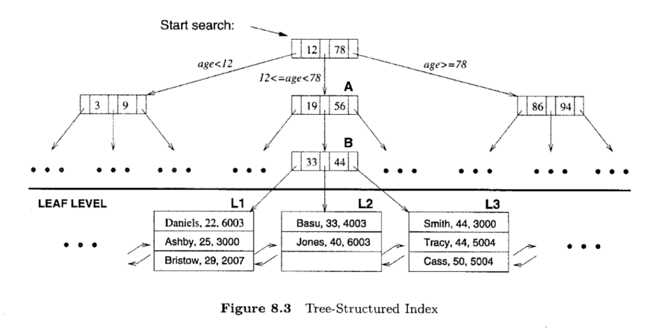
- tree-based index: B+ tree
- nodes contain pointers to lower levels
- leaves contain data entries
- B+ tree maintains a short path from root to leaf, minimising I/Os
- good for range selections
- choosing an index depends on the needs of the database: if selection queries are frequent, building an index is important. The type of index you choose will depend on the type of queries that are performed
11. Query Processing
Query Processing
- some DB operations are expensive
- clever implementation can result in $10^6$ performance improvement
- tools:
- clever implementation techniques for operators
- exploit equivalencies of relational operators
- use cost models to choose between alternatives
Relational Operations
Selection
- multiple predicates:
- a B+ tree index matches predicates that involve attributes in a prefix of the search key.
- e.g. Index on
<a,b,c>:- matches predicates on
(a,b,c), (a, b)and(a) - matches
a = 5 AND b = 3 - does not match
b = 3 - only matching predicates are used to determine cost
- matches predicates on
- e.g. index on
<a, b>: Can this be used to estimate cost of following conditions?a > x: yesa > x AND b > y: yesb > y: noa = 5 AND b = 3 & c = 7: yes. Only the first two are matching predicates.
- approach:
- find cheapest access path: index/file scan with lowest estimated page I/O
- retrieve tuples using it: predicates that match the index reduce the number of tuples retrieve, and impact the cost
- apply predicates that don’t match the index later on, on-the-fly, in
memory
- doesn’t affect total number of tuples/pages fetched
Projection
- issue: removing duplicates is expensive
- approaches: hashing, sorting
- sorting:
- scan whole relation, extract only needed attributes
- sort the result set (external merge sort)
- remove adjacent duplicates
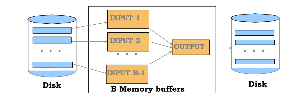
External Merge Sort
- used when data doesn’t fit in memory all at once
- conduct several passes:
- sort runs: make each of B pages individually sorted (runs)
- merge runs: make multiple passes to merge runs
Sort-based Projection
Cost =  ReadTable +             # read entire table, keep projected attributes
        WriteProjectedPages +   # write back to disk
        SortingCost +           # external merge sort
        ReadProjectedPages      # discard adjacent duplicates

WriteProjectedPages = NPages(R) * PF
SortingCost = 2*NumPasses*ReadProjectedPages
- projection factor PF: how much we are projecting, ratio with respect to
all attributes
- e.g. keeping 10% of all attributes
Hash-based projection
- scan R, extract needed attributes
- hash data into buckets: apply hash function
h1to choose one ofBoutput buffers - remove adjacent duplicates from a bucket
- 2 tuples from different partitions guaranteed to be distinct
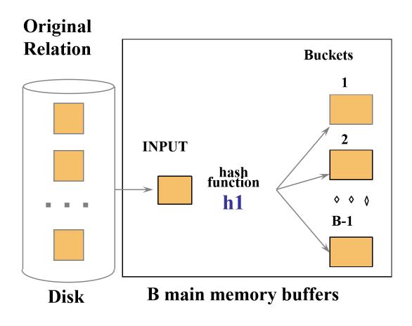
- external hashing
- partition data into B-1 partitions with hash function
h1 - load each partition, hash it with a different hash function
h2and eliminate duplicates
- partition data into B-1 partitions with hash function
Cost = ReadTable + WriteProjectedPages + ReadProjectedPages
12. Query Processing II
Joins
- very common
- can be very expensive (cross product in worst case)
- in expression $R\times S$:
- $R$: left/outer
- $S$: right/inner
- properties
- commutative: $A\times B = B\times A$
- associative: $A\times(B\times C) = (A\times B) \times C$
Simple nested loop join
- $R\bowtie S$
- for each tuple in outer relation $R$, we scan entire inner relation $S$
for each tuple r in R:
  for each tuple s in S:
    if ri = sj:
       add <r, s> to the result
Cost(SNLJ) = NPages(Outer) + NTuples(Outer) * NPages(Inner)
Page-Oriented Nested Loop Join
- $R\bowtie S$
- for each page of R, get each page of S.
- Write out matching pairs of tuple
<r, s>
- Write out matching pairs of tuple
for each page b_r in R:
  for each page b_s in S:
    for each tuple r in b_r:
      for each tuple s in b_s:
        if r_i = s_j, add <r,s> to the result
Cost(PNLJ) = NPages(Outer) + NPages(Outer) * NPages(Inner)
Block Nested Loop Join
- exploit additional memory buffers
- use one page as input buffer for scanning inner S
- use one page as output buffer
- use all remaining pages to hold block of outer R
for each block in R:
  for each page in S:
    for each matching tuple r in R-block, s in S-page:
      add `<r, s>` to result
Cost(BNLJ) = NPages(Outer) + NBlocks(Outer)*NPages(Inner)
Sort-Merge Join
- sort R and S on the join column
- scan them to do a merge
- output result tuples
- useful when:
- one/both inputs are already sorted on join attributes
- output required to be sorted on join attributes
Cost(SMJ) = Sort(Outer) + Sort(Inner)     # Sort inputs
          + NPages(Outer) + NPages(Inner) # Merge inputs

Sort(R) = external sort cost = 2*NumPasses*NPages(R)
Hash Join
- partition both relations using hash function
h: tuples from R in partition 1 can only match tuples from S in partition 1 - read in a partition of R, hash with a different hash function
h2- scan matching partition of S and probe the hash table for matches
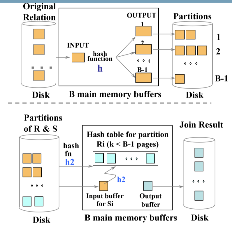
Cost(HJ) = 2*NPages(Outer) + 2*NPages(Inner)  # Create partitions
            + NPages(Outer) + NPages(Inner)   # Match partitions
General Joins
- equality over several attributes
- for sort-merge and hash join, sort/partition on combination of the join columns
- range/inequality conditions
- hash join, sort merge join not applicable
- block NL likely to be best join method here
13. Query Optimisation
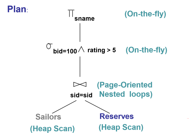
Query plan
- tree with relational algebra operators as nodes
- pipeline of tuples from bottom to top
- exclude cost of writing result, as this will be identical for all plans
- each operator labeled with choice of algorithm
Query optimisation steps
- break query into blocks
- convert block to relational algebra
- consider alternative query plans for each block
- select plan with lowest estimated cost
Break query into blocks
- query block: any statement starting with select
- unit of optimisation
- inner most block optimised first, then move outwards
Relational algebra equivalences
- Selections
Cascade
\[\sigma_{c_1 \wedge ... \wedge c_n}(R) = \sigma_{c_1}(...(\sigma_{c_n}(R)))\]Commute
\[\sigma_{c_1}(\sigma_{c_2}(R)) = \sigma_{c_2}(\sigma_{c_1}(R))\]- Projections
Cascade
\[\pi_{a_1}(R) = \pi_{a_1}(...(\pi_{a_n}(R)))\]Where $a_i$ is a set of attributes of R and $a_i \subseteq a_i+1$ for $i = 1..n-1$
-
projection also commutes with selection that only uses attributes retained by the projection
-
Joins
Associative \(R\bowtie (S \bowtie T) = (R\bowtie S)\bowtie T\)
Commutative \(R\bowtie S = S\bowtie R\)
- consequences:
- allow you to push down selections and projections before joins
- care needed for projection
- allows you to choose different join order, and pick minimum cost option
- allow you to push down selections and projections before joins
Statistics and Catalogs
- system catalog provides optimiser with information about relations and indexes
- typically contains:
- number of tuples, number of pages per relation
- number of distinct keys for each index/attribute
- low/high values
- index height
- number of index pages
- statistics are updated periodically
Cost Estimation
- for each plan, estimate the cost:
- estimate result size for each operation in tree
- estimate cost of each operation in tree
Reduction Factors
| Condition | Reduction Factor |
|---|---|
| col = value | $\frac{1}{\text{NKeys(col)}}$ |
| col > value | $\frac{\text{High(col)}-\text{value}}{\text{High(col)}-\text{Low(col)}}$ |
| col < value | $\frac{\text{value}-\text{Low(col)}}{\text{High(col)}-\text{Low(col)}}$ |
| Col_A = Col_B (join) | $\frac{1}{\max{(\text{NKeys}(Col_A), \text{NKeys}(Col_B))}}$ |
| no info | Use magic number 1/10 |
14. Query Optimisation 2
Single-relation plans
- each available access path (file scan/index) is considered
- choose lowest cost option
- heap scan is always available
- indexes are alternatives if they match selection predicates
- other operations may be performed on top of access but they don’t typically incur additional cost as they are done on the fly (e.g. projection, non-matching predicates)
Multi-relation plans
- select order of relations
- select join algorithm for each join
- for each input relation select access method (heap scan, …)
- restrict plan space to left-deep join trees
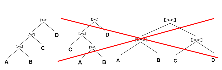
- allows you to pipeline results from intermediate operations: you don’t write back to disk, and then incur cost when you need to read again, you just feed it into the next operation
- prune plans from the tree with cross products immediately
15. Normalisation
Motivation for Normalisation

- anomalies in denormalised data
- insertion: cannot add new course until at least one student is enrolled
- deletion: if student 425 withdraws, the course is lost
- update: if the fee changes for a course, every row referencing that course will have to be updated. It would be easy to make inconsistent changes: if the fee changes for a course, every row referencing that course will have to be updated. It would be easy to make inconsistent changes.
- normalisation: technique to remove undesired redundancy from databases by breaking a large table into several smaller tables
- a relation is normalised if all determinants are candidate keys
Functional dependency
- functional dependency: set of attributes $X$ **determines $Y$ if each value of $X$
is associated with only one value of Y
- $X\rightarrow Y$: X determines Y; if I know X, then I also know Y
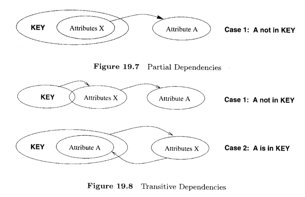
Consider A(X PK, Y PK, Z, D):
- determinants: $X, Y \rightarrow Z$
- X, Y are determinants
- key/non-key attributes: each attribute is/isn’t a part of the primary key
- partial functional dependency: $Y\rightarrow Z$
- functional dependency of 1+ non-key attributes upon part (not all) of primary key
- presence indicates normalisation required
- transitive dependency: $Z\rightarrow D$
- functional dependency between 2+ non-key attributes
Armstrong’s Axioms
- functional dependency between 2+ non-key attributes
Steps in Normalisation
- 1st Normal Form: keep atomic data
- atomic columns: cells have a single value
- in 1NF if every field contains only atomic values, i.e. no lists or sets
- 2nd Normal Form: remove partial dependencies
- in 2NF non-key attribute cannot be identified by part of a composite key
- 3rd Normal Form: remove transitive dependencies
- in 3NF non-key attribute cannot be identified by another non-key attribute
Normalisation vs Denormalisation
- normalisation:
- minimal redundancy
- allows users to insert, modify, delete rows without errors/inconsistencies
- denormalisation:
- improved query speed and performance. Good for time-critical operations
- extra work on updates to ensure data is consistent
16. Database Administration
- capacity planning: estimating disk space, transaction load
- backup and recovery: failures, responses, backups
Capacity Planning
- capacity planning: predicting when future loads will saturate the system
- determining cost-effective way of delaying saturation as much as possible
- database implementation: need to consider, both at go-live and through-life
- disk space requirements
- transaction throughput (transaction/unit time)
- will be a consideration at system design phase, and system maintenance phase
- many vendors sell capacity planning tools, which all function in a similar manner
Transaction load
- how often will each business transaction run?
- what SQL statements run for each transaction?
Storage requirements
- treat DB size as sum of all table sizes
table size = number of rows * avg row width- MySQL data type sizes
- estimate table growth rate
- use system analysis to determine growth rate of tables over time
- project total storage requirements over time
- note this is a rough estimate. Haven’t accounted for size of indexes, …
Backup and Recovery
Motivation
- backup: copy of data
- data can become corrupted, deleted, held to ransom
- backup allows restoration
- backup and recovery strategy needed
- how to back up data
- how to recover data
- backups protect from:
- human error: accidental deletion
- hardware/software malfunction: bugs, hard drive failure, memory failure
- malicious activity: security compromise
- disasters: flood, terrorist attack
- government regulation: historical archiving, privacy
Failure
Some failure categories include:
- statement failure: syntactically incorrect
- no backup required
- user process failure: process doing the work fails. Restart the application.
- no backup required
- transactions should handle issues with atomic operations
- network: connection lost etc.
- no backup required, re-establish connection
- user error: accidental drop table
- backup required
- memory failure: primary memory fails, becomes corrupt
- backup may be required
- media failure: disk failure, corruption, deletion
- backup required
Backup Taxonomy
Physical vs Logical
- physical: raw copies of files and directories, including logs
- suitable for large databases needing fast recovery
- DB preferably offline (cold backup) when backup occurs
- only portable to machines with similar configuration
- to restore:
- shut down DBMS
- copy backup over current structure on disk
- restart DBMS
- logical: backup completed through SQL queries
- slower than physical backup: SQL select vs OS copy
- output larger than physical
- doesn’t include log/config files: this may be important! e.g. for a bank
- portable: machine independent
- server available during backup
- creating backup with mySQL:
mysqldump,SELECT ... INTO OUTFILE - restore process:
mysqlimport,LOAD DATA INFILE
Online vs Offline Backup
- online, hot: backup occurs when DB is live
- clients unaware backup in progress
- needs appropriate locking to ensure data integrity
- offline, cold: DB is stopped for backup
- to prevent disrupting availability, backup could be taken from a replication server while other servers remain live
- simpler to perform
- preferable, but not always possible (e.g. when downtime cannot be tolerated)
Full vs Incremental Backup
- full: complete DB is backed up, whether physical/logical, online/offline
- includes everything needed to get DB operational in event of a failure
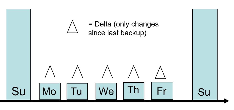
- incremental only changes since last backup are backed up
- for most DBs this means backup log files
- to restore:
- stop DB, copy backup up log files to disk
- start DB and tell it to redo the log files
Onsite vs Offsite Backup
- offsite: store copy of backup offsite
- enables disaster recovery, as backup is not physically near disaster site
- e.g. backup tapes stored in vault, backup to cloud, remote mirror databases maintained via replication
Backup Policy
- strategy: usually combination of full and incremental backups
- e.g. weekly full backup, weekday incremental backup
- conduct backups when load is low
- if using replication: use mirror DB for backups to negate performance concerns with primary DB
- test backup and restore process before it is needed
17. Transactions
Transactions
transaction: logical unit of work
- indivisible/atomic: must be either fully completed or else aborted
- DML statements are atomic
- successful transaction changes database from one consistent state to another, i.e. all data integrity constraints are satisfied
- DBMS provides user-defined transactions: sequence of DML statements
- solve 2 problems:
- need to define unit of work
- concurrent access
Defining a unit of work
- users need method to define unit of work
- transaction: multiple SQL statements embedded within larger application
- needs to be indivisible
- in case of error:
- SQL statements already completed need to be reversed
- pass error to user
- when ready, user can retry transaction
- e.g. withdrawal from a bank:
SELECT: get starting account balanceINSERT: insert detailed representation of the withdrawalUPDATE: update account balance
- MySQL implementation:
BEGIN, COMMIT, ROLLBACK
START TRANSACTION;  # also BEGIN
  # <SQL statements>
COMMIT;          # commit whole transaction
ROLLBACK;       # undoes everything
ACID: Transaction properties
- atomicity: transaction is a single, indivisible, logical unit of work
- all operations within the transaction must be completed, otherwise the transaction must be wholly aborted
- consistency: constraints holding before transaction also need to hold after it
- multiple users accessing same data see same value
- isolation: changes during execution cannot be seen by other transaction until
completed
- as the change could be rolled back, this prevents others acting on invalid data
- durability: once complete, changes made by a transaction are permanent and recoverable if system fails
Concurrent Access
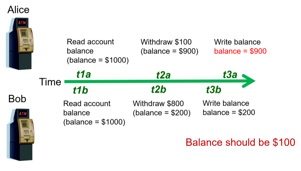
- multiple users accessing database at same time, can produce
- lost updates: Alice and Bob read account balance near simultaneously, then withdraw money. Alice and Bob are both unaware of the other person’s withdrawal. Whoever submits the update to account balance first will have the value overwritten by the other persons update, and the account balance won’t have the expected value
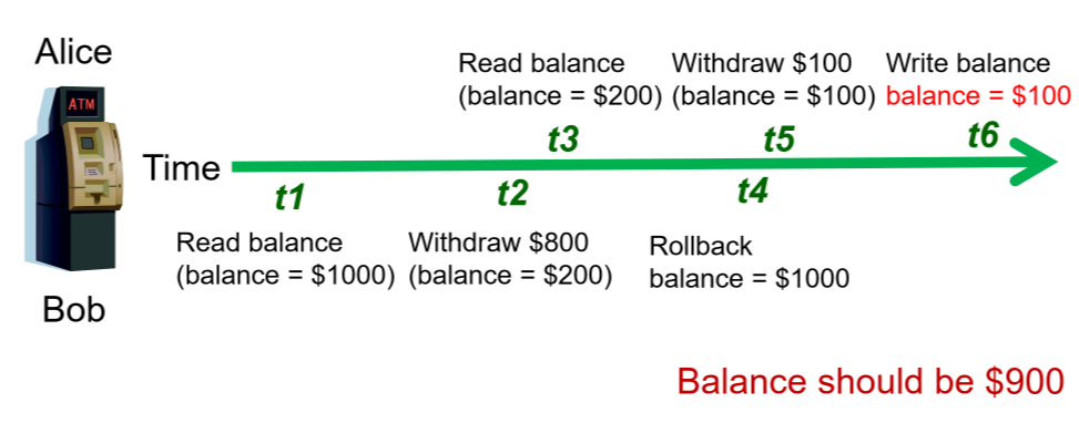
- uncommitted data: two transactions execute concurrently. The first is rolled back after the second has already accessed it.
- inconsistent retrieval: one transaction calculates aggregate over set of data, during which time other transactions update the data. Some data may be read before the change, others after the change, producing inconsistent results
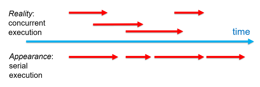
Serialisability
- ideally transactions can be serialised, such that multiple concurrent transactions
appear as if they execute one after the other
- this ensures consistency
- very expensive: lots of time because blocking unnecessarily
Concurrency Control Methods
- DBMS creates schedule of read/write operations for concurrent transactions
- interleave execution of operations with concurrency control algorithms
- methods:
- locking: primary method
- timestamping
- optimistic
Locking
- lock: guarantee exclusive use of data item to current transaction
- prevents another transaction from reading inconsistent data
- T1 acquires lock prior to data access
- lock released once transaction complete
- T2 cannot access data until lock us available
- lock manager: responsible for assigning, policing locks
Lock Granularity
- database-level: entire database locked
- good for batch processing
- unsuitable for multi-user DBMS
- T1, T2 cannot access same DB concurrently, even if they are accessing different tables
- SQLite, Access
- table-level: entire table locked
- similar to above, but not as bad
- T1, T2 can access same DB concurrently as long as they are working on different tables
- bottlenecks still exist if transactions want to access different parts of the table and wouldn’t interfere with one another
- not suitable for highly multi-user DBMS
- page-level: lock set of tuples on a disk page
- not commonly used
- row-level: allow concurrent transaction to access different rows of same
table, even if located on same page
- good availability
- high overhead: each row has a lock that must be read and written to
- most popular approach: MySQL , Oracle
- field-level: concurrent access to same row as long as accessing different attributes
- most flexible
- extremely high overhead
- not commonly used
Lock types
- binary lock: locked (1), unlocked(0)
- handles lost update problem: lock not released until statement completed
- too restrictive to yield optimal concurrency: locks even for 2
READs
- exclusive and shared lock
- exclusive: access reserved for transaction that locked it
- must be used for transaction intending to
WRITE - granted iff no other locks (exclusive or shared) held on the data item
- MySQL:
SELECT ... FOR UPDATE
- must be used for transaction intending to
- shared: grant
READaccess- transaction wants to
READdata, and no exclusive lock is held on the item - multiple transactions can have shared lock on same data if they are all just reading it
- MySQL:
SELECT ... FOR SHARE
- transaction wants to
- exclusive: access reserved for transaction that locked it
Deadlock
- deadlock: when 2 transactions wait for each other to unlock data
- T1 locks X, wants Y
- T2 locks Y, wants X
- could wait forever if not dealt with
- only happens with exclusive locks
- handle by:
- prevention
- detection
Timestamping
- timestamp: assign globally unique timestamp to each transaction
- each data item accessed by the transaction gets the timestamp
- thus for every data item, the DBMS knows which transaction performed last read/write
- when transaction wants to read/write, DBMS compares timestamp with timestamp already attacked to item and decides whether to allow access
Optimistic
- based on assumption that majority of DB operations do not conflict
- transaction executed without restrictions/checking
- when ready to commit: DBMS checks whether it/any of data it read has been altered
- if so, rollback
Transaction Log
- allows restoration of database to previous consistent state
- DBMS tracks all updates to data in transaction log:
- record for beginning of transaction
- for each SQL statement:
- operation (update, delete, insert)
- objects affected
- before/after values
- pointers to previous/next transaction log entries
- commit/ending of transaction
- also allows restoration of corrupted database
18. Data Warehousing
Data Warehousing
Motivation
- relational databases used to run day-to-day business operations
- automation of routine business processes: accounting, inventory, sales, …
- problems:
- too many of them: each department has multiple, often of different types
- produces many of the problems databases are meant to solve:
- duplicated, inaccessible, inconsistent data
- managers want data for analysis and decision making
- need means to get integrate all organisational data: informational database,
rather than transactional database
- allows all of organisation’s data to be stored in manner that supports organisational decision processes
- end user is not writing to it, just reading from it
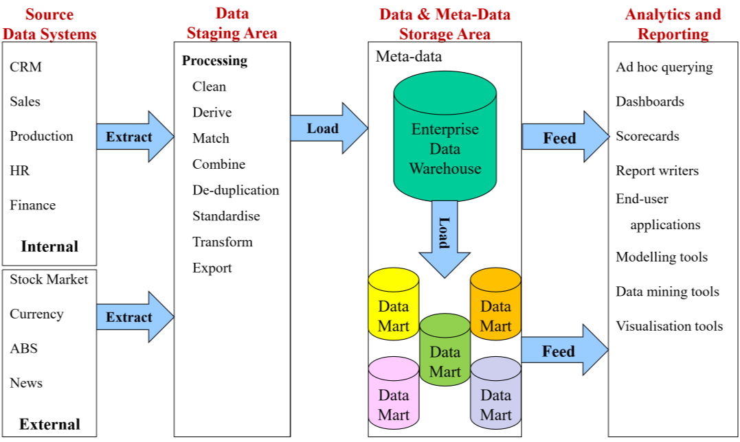
- data warehouse: single repository of organisational data
- integrates data from multiple sources
- extracts data from source systems, transforms, loads into warehouse
- makes data available to managers to support analysis and decision making
- large data store ~ TB-PB
Analytical Queries
- operational questions: e.g. Customer service: help I forgot my membership card
- typically references small number of tables
- analytical questions: e.g. campaign management: how many customers purchased $x of products in Melbourne stores?
- typically references large number of tables
- data warehousing supports analytical queries
- numerical aggregations: how many? average? total cost?
- attempting to understand relative to dimensions: sales by state by customer type
DW Characteristics
- subject oriented: organised around subjects (customers, products, sales)
- validated, integrated data:
- data from different systems converted to common format allowing comparison and consolidation
- data is validated
- time variant: stores historical data
- trend analysis
- data is a series of time-stamped snapshots
- non-volatile
- users have read only access
- updating done automatically by Extract/Transform/Load process, periodically by DBA
- allow you to:
- build Business Intelligence dashboard
- perform advanced analysis
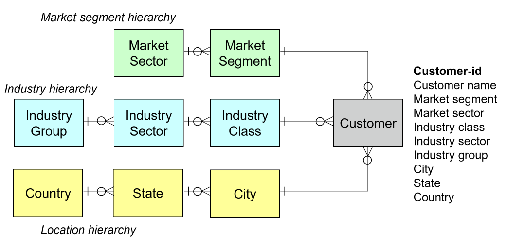
Dimensional Modelling
e.g. How much revenue did product G generate in the last 3 months, broken down by month for south easter sales region, by individual stores, broken down by _promotions, compared to estimates and to the previous product version
-
dimensional analysis: supports business analyst view
- Revenue per product per customer per location
- fact: revenue
- dimensions: product, customer, location
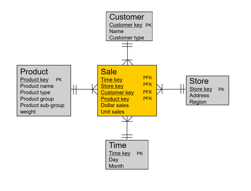
Dimensional model
- dimensional model: simple, restricted ER model
- fact table: contains business measures/facts, with FKs pointing to dimensions
- these are the values the manager is interested in
- granularity: level of detail; e.g. time period months/days
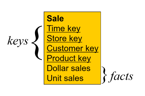
- dimensional tables: captures factor by which fact can be described/classified
- sometimes hierarchies in dimensions
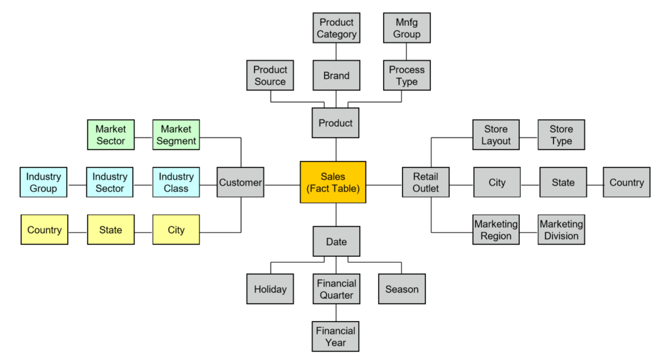
- star schema
Designing a dimensional model
- choose a business process (subject)
- choose measured facts (usually numeric, additive quantities)
- choose granularity of fact table
- choose dimensions
- complete dimension tables
Embedded Hierarchies
Snowflake schema
Denormalisation
- DW is typically denormalised
- denormalised produces:
- fewer tables
- fewer joins
- faster queries
- design tuned for end-user analysis
- data is read only and consistent from ETL process, so no risk of anomalies from unnormalised DB
19. Distributed Databases
Distributed Databases
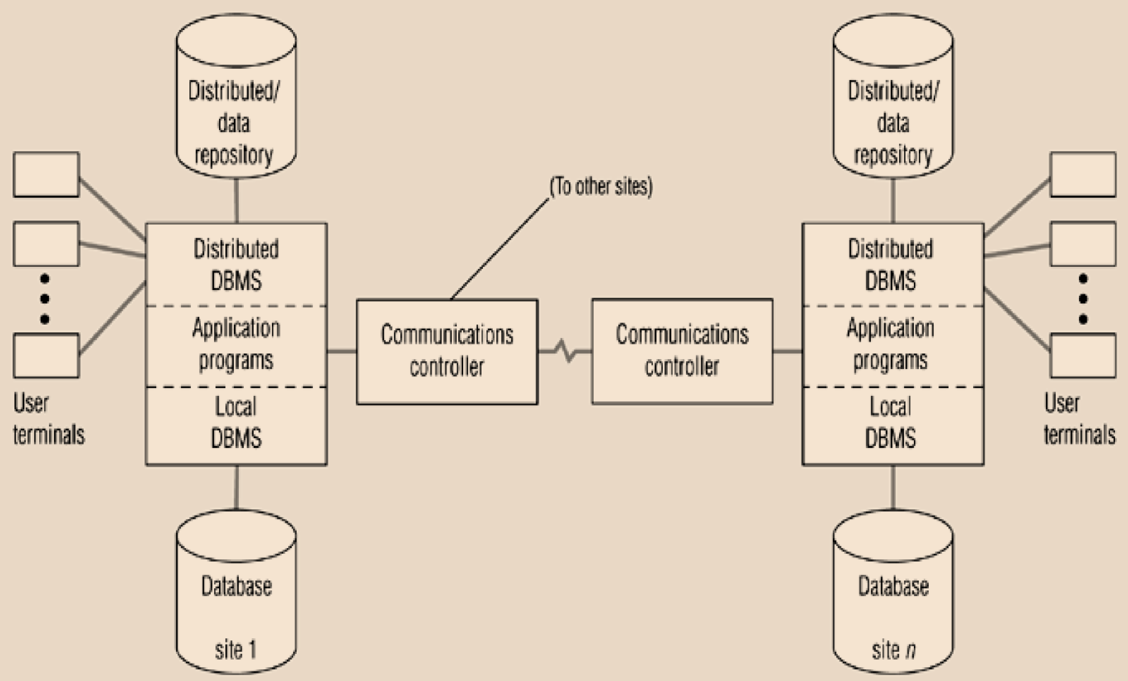
- distributed database: single logical database physically spread across multiple
computers in multiple locations, all connected via data communications link
- appears to user to be a single database
- focus here
- decentralised database: collection of independent databases which are not
networked together as one logical database
- users see many databases
- physical servers have their own internal memory structures
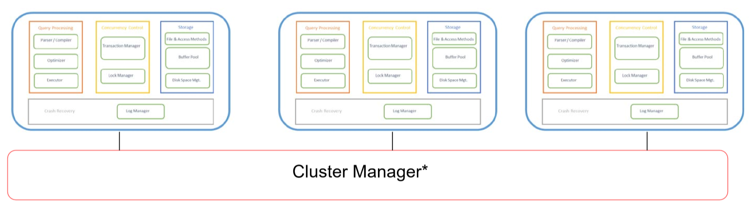
- cluster manager: coordinates communication between physical servers
Advantages
- good fit for geographically distributed organisations/users
- data can be located near sites with greatest demand: e.g. store sport info near the point of interest: AFL - Melbourne, NFL - New York, etc.
- faster data access (for local data)
- faster data processing: workload shared between physical servers
- modular growth: add new servers as load increases
- increased reliability/availability: less likely to have single point of failure
- supports database recovery: data is replicated across sites
Disadvantages
- complexity of management and control
- who/where is current version of record?
- who is waiting to update information?
- how does this get displayed to user?
- data integrity: additional exposure to improper updating
- simultaneous updates from different locations: which should be chosen?
- solutions:
- transaction manager
- master-slave design: master allowed to write, slaves read only
- security: many server sites means higher risk of breach
- protection needed from cyber and physical attacks
- lack of standards: different RDDBMS vendors use different protocols
- training/maintenance costs: more complex IT infrastructure
- increased disk storage ($)
- fast intra/inter network infrastructure ($$$)
- clustering software (\(\))
- network speed (\(\)$)
- increased storage requirements: replication
Objectives and Trade-offs
- location transparency: user doesn’t need to know where data are stored
- requests to retrieve/update data from any site are forwarded by the system to theX relevant site for processing
- all data in the network appears as a single logical database stored at a single site as far as the user can tell
- a single query could join data from tables in multiple sites
- local autonomy: node can continue to function for local users if connectivity lost
- users can administer local database: local data, security, log transactions, recovery
- trade-offs:
- availability vs consistency: DB may be unavailable while updating, but more consistent
- synchronous vs asynchronous update
- e.g. banking: synchronous; social networks: asynchronous
Distribution Options
- some combination of below options is also typical
Data Replication
- data replication: data copied across sites
- advantages
- currently popular approach for high availability global systems: implemented by most SQL and NoSQL DBs
- high reliability: redundant copies of data
- fast access at location where most accessed
- can avoid complicated distributed integrity routines, with replicated data being refreshed at specified intervals
- if a node goes down availability is largely unaffected
- reduced network traffic at prime time if updates can be delayed
- need more storage space: each server stores a copy of each tuple
- disadvantages
- may need to be tolerant of out-of-date data
- updates could cause performance problems for busy nodes
- takes time for update operations
- updates place heavy demand on networks, and high speed networks are expensive
Synchronous Update
- e.g. for banking
- data continuously kept up to date: users anywhere can access data and get the same answer
- if any copy of a data item is updated, the same update is applied immediately to all other copies, otherwise it is aborted
- ensures data integrity
- minimises complexity of knowing where more recent copy of data is
- slow response time, high network usage: time taken to check update accurately and completely propagated
Asynchronous Update
- e.g. for social network
- delay in propagating data updates to remote databases
- application able to tolerate some degree of temporary inconsistency
- acceptable response time: updates happen locally; replicas are synchronised in batches and predetermined intervals
- more complex to plan/design: need to get right level of data integrity/consistency
- suits some systems more than others
Horizontal Paritioning
- horizontal partitioning: table rows distributed across sites
- advantages:
- data stored close to where its used
- local access optimisation: better performance
- only relevant data stored locally: good for security
- combining data: unions across partitions c.f. joins for vertical partitioning: unions are less expensive
- disadvantages
- accessing data across partitions: inconsistent access speed
- no data replication: backup vulnerability
- in practice: typically have partial replication across sites
Vertical partitioning
- vertical partitioning: table columns distributed across sites
- advantages/disadvantages mostly the same as for horizontal partitioning
- disadvantage:
- combining data: joins across partitions, more expensive c.f. horizontal partitions
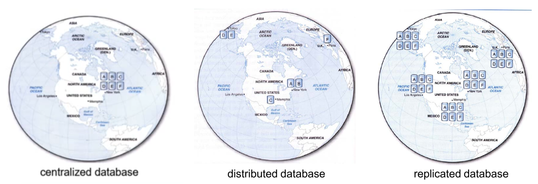
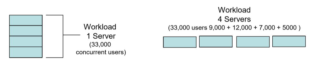
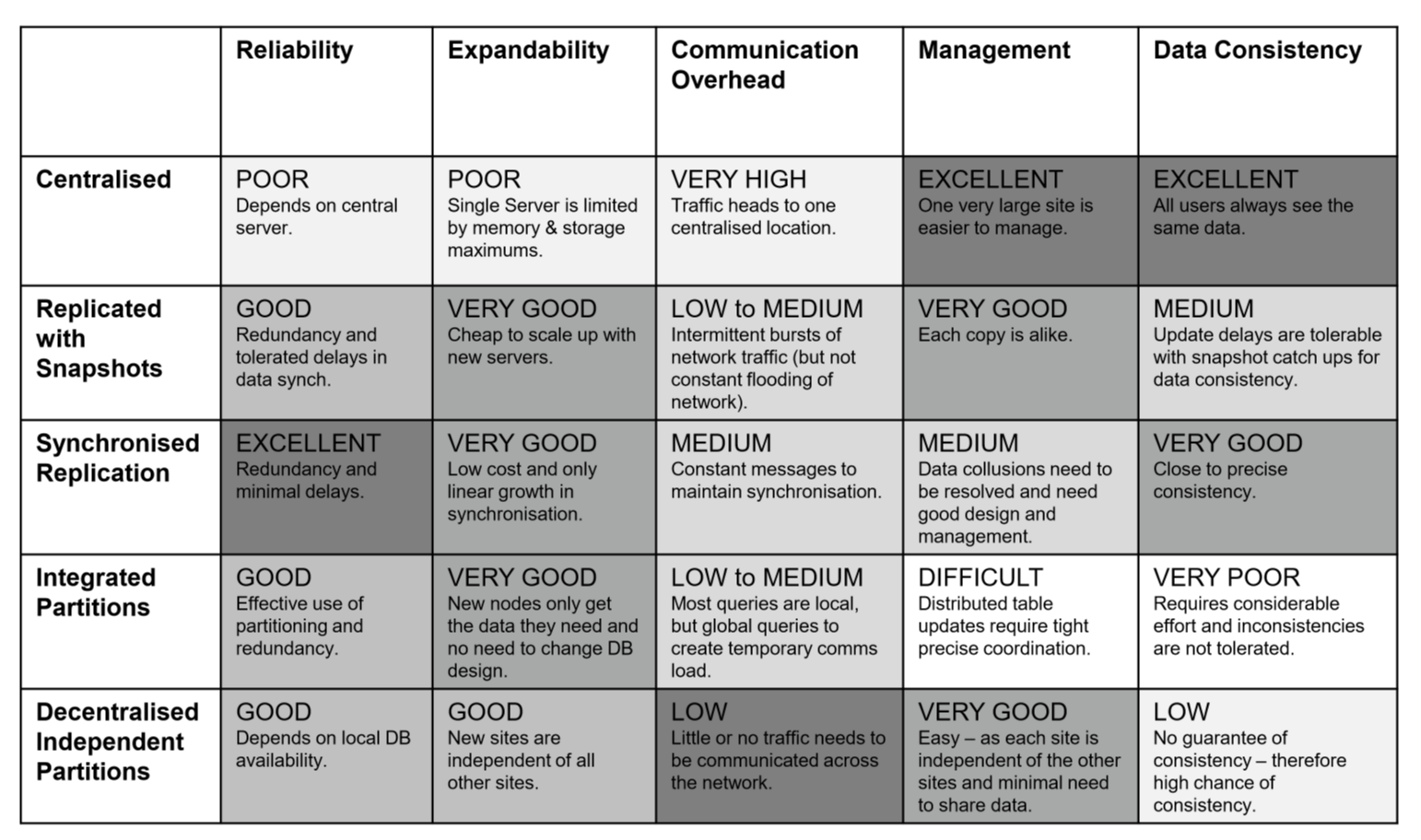
Comparing configurations
- Centralised DB, distributed access:
- DB at one location accessed from everywhere
- Replication with periodic asynchronous snapshot update
- DB at many locations, with each copy updated periodically
- replication with near real-time synchronisation of updates
- DB at many locations, each copy updated in nreal real-time
- partitioned, integrated, one logical database
- DB partitioned across many sites within a logical DB and single DBMS
- partitioned, independent, non-integrated segments (decentralised)
- data partitioned across many sites
- independent, non-integrated segmented
- multiple DBMS
Functions of a distributed DBMS
- locate data with distributed catalog (statistics + metadata)
- determine location from which to retrieve data and process query components
- translate between nodes with different local DBMS
- data consistency
- global primary key control
- provide scalability, security, concurrency, query optimisation, failure recovery
Date’s 12 Commandments for Distributed Databases
- represent a target for DDBMS, while most don’t satisfy all principles
Independence
- Local site independence: each local site can act as an independent, autonomous, DBMS. Each site is responsible for security, concurrency, control, backup, recovery.
- Central site independence: no site in the network relies on a central site, or on any other site. Each site has the same capabilities.
- Failure independence: system is not affected by node failures. The system is in continuous operation, even in the case of a node failure, or expansion of the network.
- Hardware independence
- Operating System independence
- Network independence
- Database independence
Transparency
- Location transparency: user doesn’t need to know location of data to retrieve it
- Fragmentation transparency: data fragmentation is transparent to the user, who sees only one logical database.
- Replication transparency: user sees only one logical database. DDBMS transparently selects database fragments to access.
- Distributed query processing: query may be executed at several different sites. Query optimisation is performed transparently by DDBMS.
- Distributed transaction processing: transaction may update data at several sites, and transaction is executed transparently.
20. NoSQL
Motivation for NoSQL
- relational databases, have a number of pros, which explain their dominance:
- simple, can capture most business use case
- integrate multiple applications with shared data store
- SQL, standard interface language
- ad hoc queries
- fast, reliable, concurrent, consistent
- relational databases, also have their cons:
- object-relational impedance mismatch
- poor with big data
- poor with clustered/replicated servers (when you get > $10^6$ nodes)
- NoSQL has arisen due to these cons, but relational still relevant
- often only need eventual consistency
NoSQL Goals
- reduce impedance mismatch: improve developer productivity
- big data: handle larger data volumes and throughput
Object-relational impedance mismatch
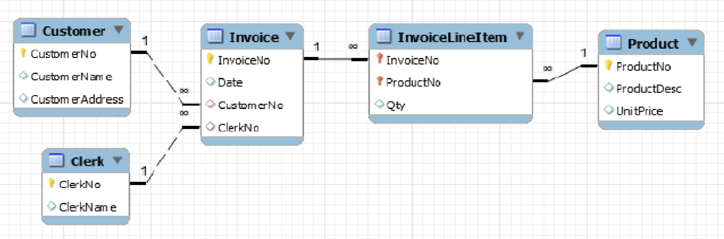
- example: invoice with a header of customer details, and a list of objects
- relational model: data stored in separate tables for order + customer + …
- cannot model real-world object directly
- lots of work to disassemble and reassemble aggregate
- object oriented model: class with composition and inheritance. All data in one place
- relational model: data stored in separate tables for order + customer + …
- Difficulty of integrating OOP with relational databases
- Objects reference one another, forming a graph (e.g. with cycles)
- Relational schema is tabular, defining linked heterogeneous tuples
Various types of mismatch, e.g.
- encapsulation: object-relational mappers necessarily expose underlying content, violating encapsulation
- accessibility: in OOP public/private is absolute characteristic of data’s state, while in relational model it is relative to need
- classes, inheritance, polymorphism: not supported by relational DB
- type system mismatch: relational model prohibits pointers. Scalar types may be vastly different.
- structural mismatch: objects composed of objects, objects specialise from a more general definition. Difficult to map onto relational schema.
- integrity mismatch: OOP doesn’t declare constraints, exception raising protection logic. Relational database requires declarative constraints.
- transactional differences: unit of work in relational DB is much larger than that in OOP
- manipulative differences: SQL vs custom OOP querying
3Vs of Big Data
- volume: much larger quantity than typical for relational DB
- variety: many different data types, formats
- velocity: data comes at high rate
Big Data Characterisitics
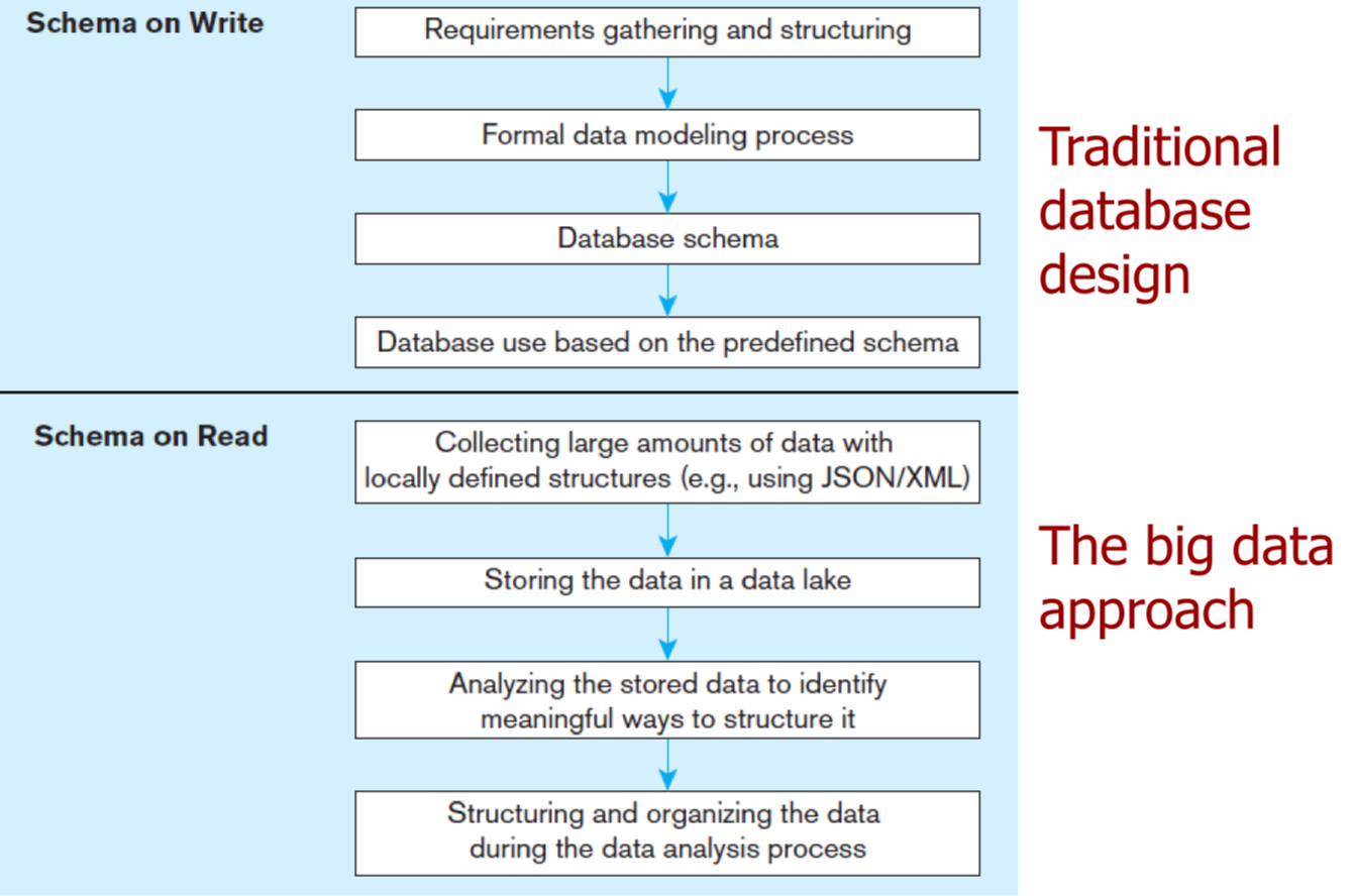
- schema on read: data model determined later, as dictated by use case (XML, JSON)
- c.f. schema on write: pre-existing data model, approach of relational DB
- capture and store data, worry about how you want to use it later
- data lake: large integrated repository for data without a predefined schema
- capture everything
- dive in anywhere
- flexible access
NoSQL Features
- doesn’t use relational model or SQL
- runs well on distributed servers
- often open source
- build for modern web
- schema-less (often has an implicit schema)
- supports schema on read
- not ACID compliant
- eventually consistent
NoSQL Variants - Aggregate oriented
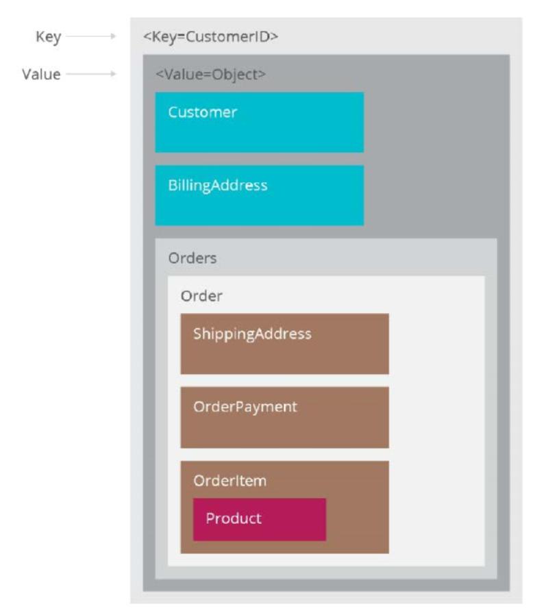
- aggregate-oriented databases store business objects in entirety
- pros
- entire data stored together. Eliminates need for transactions
- efficient storage on clusters/distributed DBs
- cons
- harder to analyse across subfields of aggregates
- e.g. sum over products instead of over orders
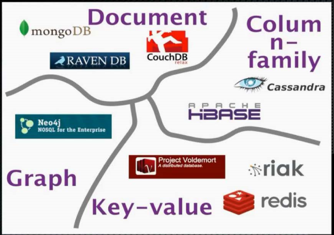
Key-value stores
- simple pair of key and associated collection of values
- database has no knowledge of structure/meaning of values
- key: primary key, usually a string
- value: anything (number, array, image, JSON)
- up to application to interpret
- operations: put, get, update
- example: Redis, DynamoDB
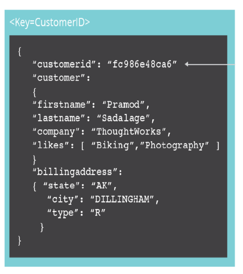
Document database
- similar to KV store, but document is structured, allow manipulation of specific elements separately
- document examinable by database:
- content can be queried
- parts of document can be updated
- document: JSON file (typically)
- e.g. MongoDb
- more structure than key-value store, easier to parse and query
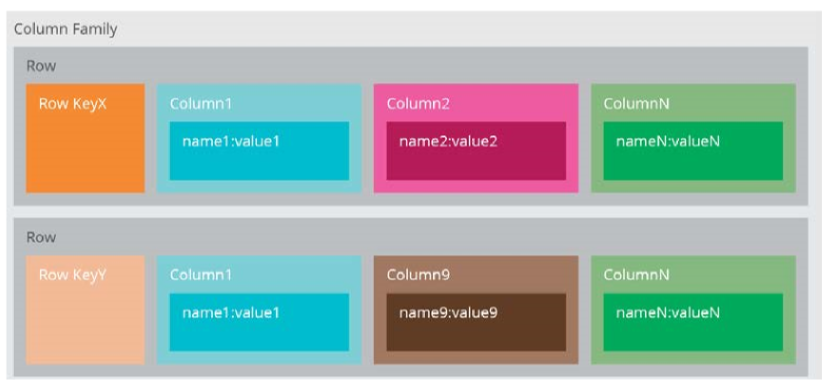
Column family
- columns stored together on disk, rather than rows, primarily for efficiency
- analysis becomes faster as less data is fetched
- automatic vertical partitioning
- related columns grouped into families
- e.g. Cassandra, BigTable
NoSQL Variants - Graph databases
- maintain information regarding relationships between data items
- nodes with properties
- e.g. friendship graph
- graphs are difficult to program in relational DB
- graph DB stores entities and their relationships
- graph queries deduce knowledge from the graph
- e.g. Neo4J
CAP Theorem
- CAP Theorem: you can only have 2 of consistency, partition tolerance, availability
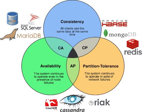
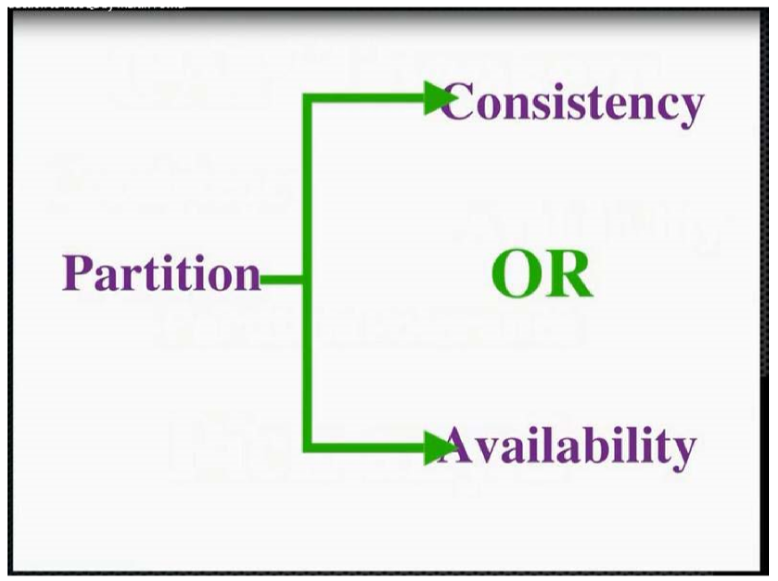
- Fowler’s version: if you have a distributed database, when a partition occurs, then choose between consistency OR availability
ACID vs BASE
- ACID: Atomic, consistent, Isolated, Durable
-
BASE: Basically available, Soft State, Eventual consistency
- basically available: requests will receive a response, but it may be inconsistent or changing
- soft state: state can change over time, even when there is no input there may be changes due to eventual consistency
- eventual consistency: system will eventually become consistent once it stops
receiving input
- data will propagate everywhere eventually but system continues to receive input and isn’t checking consistency of every transaction before proceeding